37  广义可加模型

library(mgcv)      # 广义可加模型
library(splines)   # 样条
library(cmdstanr)  # 编译采样
library(ggplot2)   # 作图
library(bayesplot) # 后验分布
library(loo)       # LOO-CV
library(rstanarm)  # 贝叶斯可加模型
library(INLA)      # 近似贝叶斯推断
options(mc.cores = 2) # 全局设置双核

相比于广义线性模型，广义可加模型可以看作是一种非线性模型，模型中含有非线性的成分。

注释

• 多元适应性（自适应）回归样条 multivariate adaptive regression splines
• Friedman, Jerome H. 1991. Multivariate Adaptive Regression Splines. The Annals of Statistics. 19(1):1–67. https://doi.org/10.1214/aos/1176347963
• earth: Multivariate Adaptive Regression Splines http://www.milbo.users.sonic.net/earth
• Friedman, Jerome H. 2001. Greedy function approximation: A gradient boosting machine. The Annals of Statistics. 29(5):1189–1232. https://doi.org/10.1214/aos/1013203451
• Friedman, Jerome H., Trevor Hastie and Robert Tibshirani. Additive Logistic Regression: A Statistical View of Boosting. The Annals of Statistics. 28(2): 337–374. http://www.jstor.org/stable/2674028
• Flexible Modeling of Alzheimer’s Disease Progression with I-Splines PDF 文档
• Implementation of B-Splines in Stan 网页文档

37.1 案例：模拟摩托车事故

37.1.1 mgcv

MASS 包的 mcycle 数据集

data(mcycle, package = "MASS")
str(mcycle)

#> 'data.frame':    133 obs. of  2 variables:
#>  $ times: num  2.4 2.6 3.2 3.6 4 6.2 6.6 6.8 7.8 8.2 ...
#>  $ accel: num  0 -1.3 -2.7 0 -2.7 -2.7 -2.7 -1.3 -2.7 -2.7 ...

library(ggplot2)
ggplot(data = mcycle, aes(x = times, y = accel)) +
  geom_point() +
  theme_classic() +
  labs(x = "时间（ms）", y = "加速度（g）")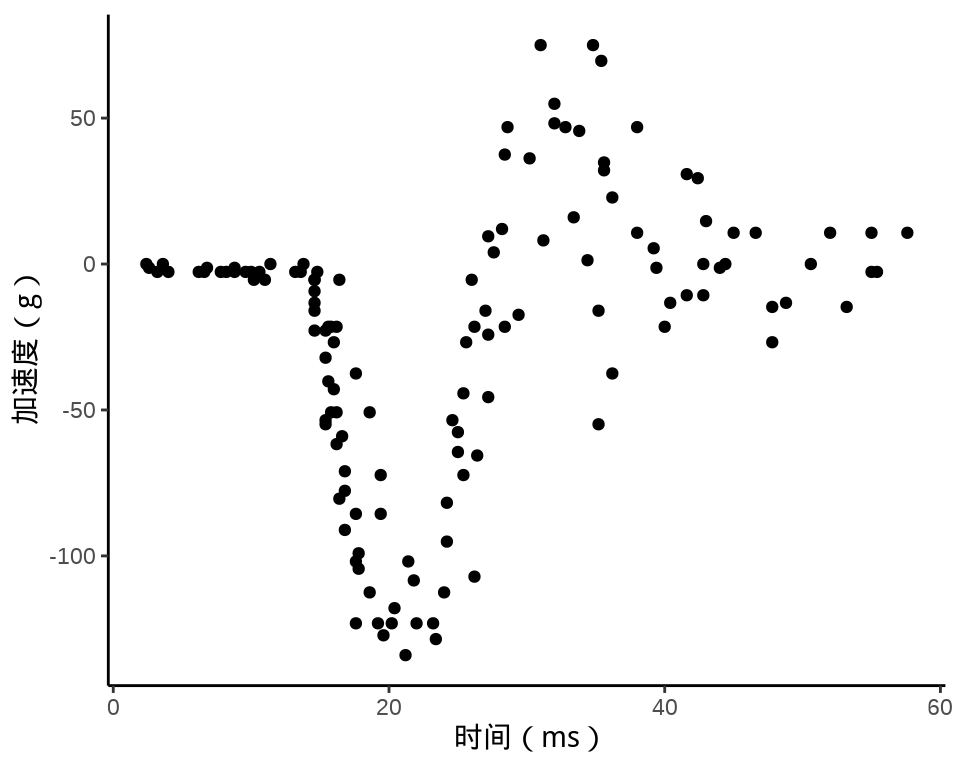

图 37.1: mcycle 数据集

样条回归

library(mgcv)
mcycle_mgcv <- gam(accel ~ s(times), data = mcycle, method = "REML")
summary(mcycle_mgcv)

#> 
#> Family: gaussian 
#> Link function: identity 
#> 
#> Formula:
#> accel ~ s(times)
#> 
#> Parametric coefficients:
#>             Estimate Std. Error t value Pr(>|t|)    
#> (Intercept)  -25.546      1.951  -13.09   <2e-16 ***
#> ---
#> Signif. codes:  0 '***' 0.001 '**' 0.01 '*' 0.05 '.' 0.1 ' ' 1
#> 
#> Approximate significance of smooth terms:
#>            edf Ref.df    F p-value    
#> s(times) 8.625  8.958 53.4  <2e-16 ***
#> ---
#> Signif. codes:  0 '***' 0.001 '**' 0.01 '*' 0.05 '.' 0.1 ' ' 1
#> 
#> R-sq.(adj) =  0.783   Deviance explained = 79.7%
#> -REML = 616.14  Scale est. = 506.35    n = 133

方差成分

gam.vcomp(mcycle_mgcv, rescale = FALSE)

#> 
#> Standard deviations and 0.95 confidence intervals:
#> 
#>            std.dev     lower      upper
#> s(times) 807.88726 480.66162 1357.88215
#> scale     22.50229  19.85734   25.49954
#> 
#> Rank: 2/2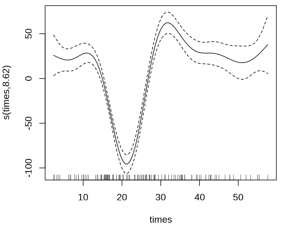

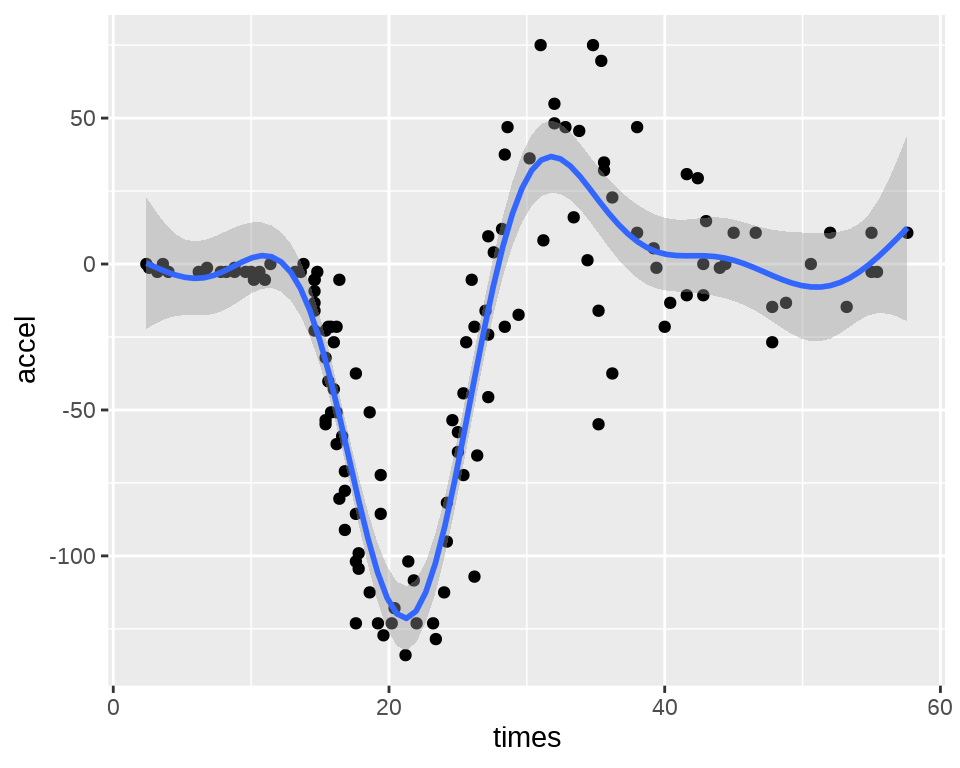
plot(mcycle_mgcv)

图 37.2: mcycle 数据集

ggplot2 包的平滑图层函数 geom_smooth() 集成了 mgcv 包的函数 gam() 的功能。

library(ggplot2)
ggplot(data = mcycle, aes(x = times, y = accel)) +
  geom_point() +
  geom_smooth(method = "gam", formula = y ~ s(x, bs = "tp"), method.args = list(method = "REML"))

图 37.3: ggplot2 平滑

37.1.2 cmdstanr

library(cmdstanr)

37.1.3 rstanarm

rstanarm 可以拟合一般的广义可加（混合）模型。

library(rstanarm)
mcycle_rstanarm <- stan_gamm4(accel ~ s(times),
  data = mcycle, family = gaussian(), cores = 2, seed = 20232023,
  iter = 4000, warmup = 1000, thin = 10, refresh = 0,
  adapt_delta = 0.99
)
summary(mcycle_rstanarm)

#> 
#> Model Info:
#>  function:     stan_gamm4
#>  family:       gaussian [identity]
#>  formula:      accel ~ s(times)
#>  algorithm:    sampling
#>  sample:       1200 (posterior sample size)
#>  priors:       see help('prior_summary')
#>  observations: 133
#> 
#> Estimates:
#>                        mean    sd      10%     50%     90%  
#> (Intercept)            -25.5     2.2   -28.3   -25.5   -22.8
#> s(times).1             340.7   237.5    33.1   336.2   645.1
#> s(times).2           -1205.4   258.8 -1538.4 -1203.4  -879.0
#> s(times).3            -574.1   153.9  -779.7  -576.7  -377.6
#> s(times).4            -617.8   139.1  -798.1  -618.1  -436.3
#> s(times).5            1060.3    85.3   951.8  1060.3  1166.1
#> s(times).6             -89.4    50.8  -154.7   -88.6   -24.8
#> s(times).7            -233.7    34.5  -277.2  -233.8  -187.9
#> s(times).8              16.1   109.2  -121.5    15.5   153.8
#> s(times).9              -0.2    33.8   -29.6     0.1    27.3
#> sigma                   24.8     1.7    22.6    24.8    26.9
#> smooth_sd[s(times)1]   402.7    61.5   325.6   399.3   482.2
#> smooth_sd[s(times)2]    24.2    24.4     2.2    16.6    57.6
#> 
#> Fit Diagnostics:
#>            mean   sd    10%   50%   90%
#> mean_PPD -25.6    3.1 -29.6 -25.6 -21.6
#> 
#> The mean_ppd is the sample average posterior predictive distribution of the outcome variable (for details see help('summary.stanreg')).
#> 
#> MCMC diagnostics
#>                      mcse Rhat n_eff
#> (Intercept)          0.1  1.0   952 
#> s(times).1           6.4  1.0  1360 
#> s(times).2           7.4  1.0  1224 
#> s(times).3           4.4  1.0  1217 
#> s(times).4           4.1  1.0  1171 
#> s(times).5           2.4  1.0  1229 
#> s(times).6           1.5  1.0  1088 
#> s(times).7           1.1  1.0  1072 
#> s(times).8           3.3  1.0  1076 
#> s(times).9           1.0  1.0  1178 
#> sigma                0.1  1.0  1006 
#> smooth_sd[s(times)1] 1.7  1.0  1255 
#> smooth_sd[s(times)2] 0.7  1.0  1191 
#> mean_PPD             0.1  1.0  1301 
#> log-posterior        0.1  1.0  1071 
#> 
#> For each parameter, mcse is Monte Carlo standard error, n_eff is a crude measure of effective sample size, and Rhat is the potential scale reduction factor on split chains (at convergence Rhat=1).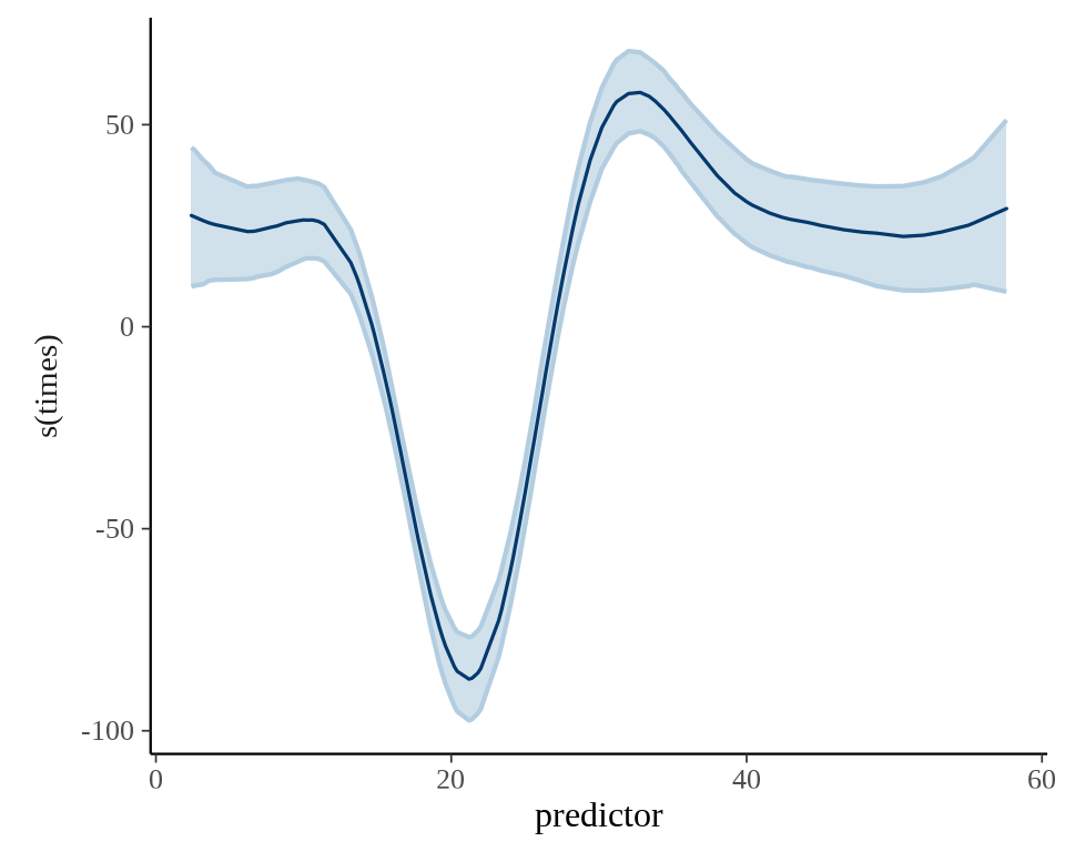

plot_nonlinear(mcycle_rstanarm)

图 37.4: 非线性部分

LOO 值

# LOO
loo(mcycle_rstanarm)

#> 
#> Computed from 1200 by 133 log-likelihood matrix
#> 
#>          Estimate   SE
#> elpd_loo   -611.4  8.7
#> p_loo         7.3  1.3
#> looic      1222.7 17.5
#> ------
#> Monte Carlo SE of elpd_loo is 0.1.
#> 
#> Pareto k diagnostic values:
#>                          Count Pct.    Min. n_eff
#> (-Inf, 0.5]   (good)     132   99.2%   533       
#>  (0.5, 0.7]   (ok)         1    0.8%   260       
#>    (0.7, 1]   (bad)        0    0.0%   <NA>      
#>    (1, Inf)   (very bad)   0    0.0%   <NA>      
#> 
#> All Pareto k estimates are ok (k < 0.7).
#> See help('pareto-k-diagnostic') for details.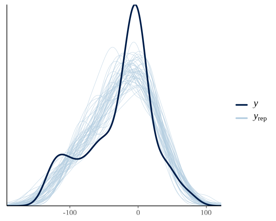

pp_check(mcycle_rstanarm)

图 37.5: 后验预测分布

37.1.4 brms

另一个综合型的贝叶斯分析扩展包是 brms 包

# 拟合模型
mcycle_brms <- brms::brm(accel ~ s(times),
  data = mcycle, family = gaussian(), cores = 2, seed = 20232023,
  iter = 4000, warmup = 1000, thin = 10, refresh = 0, silent = 2,
  control = list(adapt_delta = 0.99)
)
# 模型输出
summary(mcycle_brms)

#>  Family: gaussian 
#>   Links: mu = identity; sigma = identity 
#> Formula: accel ~ s(times) 
#>    Data: mcycle (Number of observations: 133) 
#>   Draws: 4 chains, each with iter = 4000; warmup = 1000; thin = 10;
#>          total post-warmup draws = 1200
#> 
#> Smooth Terms: 
#>               Estimate Est.Error l-95% CI u-95% CI Rhat Bulk_ESS Tail_ESS
#> sds(stimes_1)   716.18    173.55   447.43  1129.05 1.00     1208     1112
#> 
#> Population-Level Effects: 
#>           Estimate Est.Error l-95% CI u-95% CI Rhat Bulk_ESS Tail_ESS
#> Intercept   -25.42      1.97   -29.32   -21.52 1.00     1197     1214
#> stimes_1    130.28    282.27  -419.51   704.47 1.00     1070     1173
#> 
#> Family Specific Parameters: 
#>       Estimate Est.Error l-95% CI u-95% CI Rhat Bulk_ESS Tail_ESS
#> sigma    22.73      1.51    19.97    26.01 1.00     1135     1209
#> 
#> Draws were sampled using sampling(NUTS). For each parameter, Bulk_ESS
#> and Tail_ESS are effective sample size measures, and Rhat is the potential
#> scale reduction factor on split chains (at convergence, Rhat = 1).

固定效应

brms::fixef(mcycle_brms)

#>            Estimate  Est.Error       Q2.5     Q97.5
#> Intercept -25.41669   1.972042  -29.32341 -21.51916
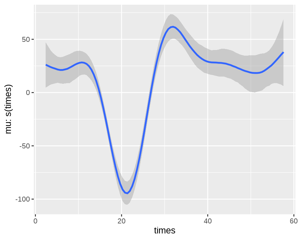
#> stimes_1  130.27592 282.265346 -419.50765 704.46677

模型中样条平滑的效应

plot(brms::conditional_smooths(mcycle_brms))

图 37.6: 样条平滑效应

LOO 值与 rstanarm 包计算的值很接近。

brms::loo(mcycle_brms)

#> 
#> Computed from 1200 by 133 log-likelihood matrix
#> 
#>          Estimate   SE
#> elpd_loo   -608.6 10.3
#> p_loo         9.1  1.6
#> looic      1217.2 20.5
#> ------
#> Monte Carlo SE of elpd_loo is 0.1.
#> 
#> All Pareto k estimates are good (k < 0.5).
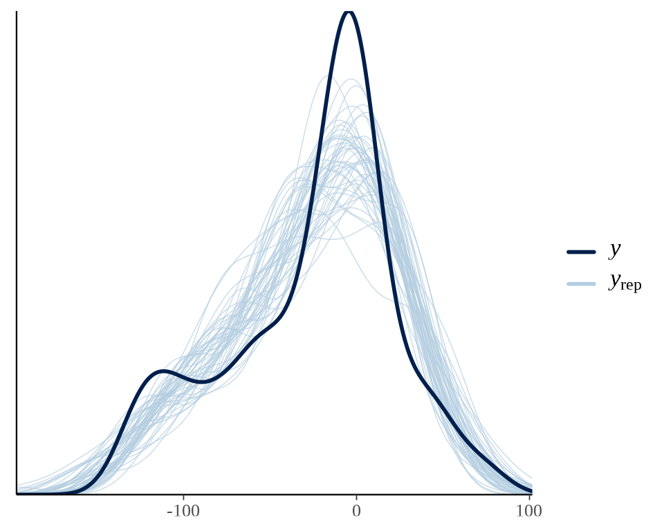
#> See help('pareto-k-diagnostic') for details.

后验预测分布检查

brms::pp_check(mcycle_brms, ndraws = 50)

图 37.7: 后验预测分布

37.1.5 GINLA

library(mgcv)
mcycle_mgcv <- gam(accel ~ s(times), data = mcycle, fit = FALSE)
# 简化版 INLA
mcycle_ginla <- ginla(G = mcycle_mgcv)
str(mcycle_ginla)

#> List of 2
#>  $ density: num [1:10, 1:100] 2.04e-04 2.13e-05 8.21e-06 3.47e-05 1.14e-05 ...
#>  $ beta   : num [1:10, 1:100] -32.8 -133.4 -139.4 -152.5 -153.3 ...

最大后验估计

idx <- apply(mcycle_ginla$density, 1, function(x) x == max(x))
mcycle_ginla$beta[t(idx)]

#>  [1]   39.378019 -110.258456  -24.618491   89.506696   -9.449407 -110.635738
#>  [7]   16.145715  -25.472566  -63.095635   35.893285

37.1.6 INLA

library(INLA)
library(splines)

37.2 案例：朗格拉普岛核污染

从线性到可加，意味着从线性到非线性，可加模型容纳非线性的成分，比如高斯过程、样条。

37.2.1 mgcv

本节复用 章节 28 朗格拉普岛核污染数据，相关背景不再赘述，下面首先加载数据到 R 环境。

# 加载数据
rongelap <- readRDS(file = "data/rongelap.rds")
rongelap_coastline <- readRDS(file = "data/rongelap_coastline.rds")

接着，将岛上各采样点的辐射强度展示出来，算是简单回顾一下数据概况。

library(plot3D)
with(rongelap, {
  opar <- par(mar = c(.1, 2.5, .1, .1), no.readonly = TRUE)
  rongelap_coastline$cZ <- 0
  scatter3D(
    x = cX, y = cY, z = counts / time, 
    xlim = c(-6500, 50), ylim = c(-3800, 110),
    xlab = "\n横坐标（米）", ylab = "\n纵坐标（米）",
    zlab = "\n辐射强度", lwd = 0.5, cex = 0.8,
    pch = 16, type = "h", ticktype = "detailed",
    phi = 40, theta = -30, r = 50, d = 1,
    expand = 0.5, box = TRUE, bty = "b",
    colkey = F, col = "black",
    panel.first = function(trans) {
      XY <- trans3D(
        x = rongelap_coastline$cX,
        y = rongelap_coastline$cY,
        z = rongelap_coastline$cZ,
        pmat = trans
      )
      lines(XY, col = "gray50", lwd = 2)
    }
  )
  rongelap_coastline$cZ <- NULL
  on.exit(par(opar), add = TRUE)
})

图 37.8: 岛上各采样点的辐射强度

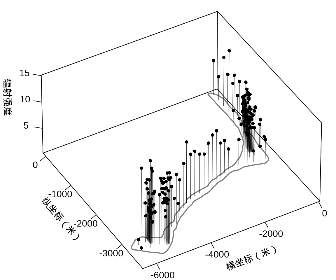
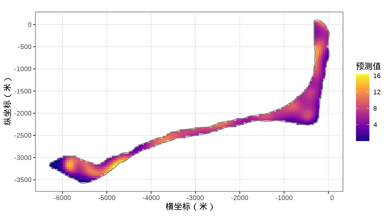
在这里，从广义可加混合效应模型的角度来对核污染数据建模，空间效应仍然是用高斯过程来表示，响应变量服从带漂移项的泊松分布。采用 mgcv 包 (S. N. Wood 2004) 的函数 gam() 拟合模型，其中，含 49 个参数的样条近似高斯过程，高斯过程的核函数为默认的梅隆型。更多详情见 mgcv 包的函数 s() 帮助文档参数的说明，默认值是梅隆型相关函数及默认的范围参数，作者自己定义了一套符号约定。

library(nlme)
library(mgcv)
fit_rongelap_gam <- gam(
  counts ~ s(cX, cY, bs = "gp", k = 50), offset = log(time), 
  data = rongelap, family = poisson(link = "log")
)
# 模型输出
summary(fit_rongelap_gam)

#> 
#> Family: poisson 
#> Link function: log 
#> 
#> Formula:
#> counts ~ s(cX, cY, bs = "gp", k = 50)
#> 
#> Parametric coefficients:
#>             Estimate Std. Error z value Pr(>|z|)    
#> (Intercept) 1.976815   0.001642    1204   <2e-16 ***
#> ---
#> Signif. codes:  0 '***' 0.001 '**' 0.01 '*' 0.05 '.' 0.1 ' ' 1
#> 
#> Approximate significance of smooth terms:
#>            edf Ref.df Chi.sq p-value    
#> s(cX,cY) 48.98     49  34030  <2e-16 ***
#> ---
#> Signif. codes:  0 '***' 0.001 '**' 0.01 '*' 0.05 '.' 0.1 ' ' 1
#> 
#> R-sq.(adj) =  0.876   Deviance explained = 60.7%
#> UBRE = 153.78  Scale est. = 1         n = 157

# 随机效应
gam.vcomp(fit_rongelap_gam)

#> s(cX,cY) 
#> 2543.376

值得一提的是核函数的类型和默认参数的选择，参数 m 接受一个向量， m[1] 取值为 1 至 5，分别代表球型 spherical, 幂指数 power exponential 和梅隆型 Matern with \(\kappa\) = 1.5, 2.5 or 3.5 等 5 种相关/核函数。

# 球型相关函数及范围参数为 0.5
fit_rongelap_gam <- gam(
  counts ~ s(cX, cY, bs = "gp", k = 50, m = c(1, .5)),
  offset = log(time), data = rongelap, family = poisson(link = "log")
)

接下来，基于岛屿的海岸线数据划分出网格，将格点作为新的预测位置。

library(sf)

#> Linking to GEOS 3.12.0, GDAL 3.7.3, PROJ 9.2.1; sf_use_s2() is TRUE

library(abind)
library(stars)
# 类型转化
rongelap_sf <- st_as_sf(rongelap, coords = c("cX", "cY"), dim = "XY")
rongelap_coastline_sf <- st_as_sf(rongelap_coastline, coords = c("cX", "cY"), dim = "XY")
rongelap_coastline_sfp <- st_cast(st_combine(st_geometry(rongelap_coastline_sf)), "POLYGON")
# 添加缓冲区
rongelap_coastline_buffer <- st_buffer(rongelap_coastline_sfp, dist = 50)
# 构造带边界约束的网格
rongelap_coastline_grid <- st_make_grid(rongelap_coastline_buffer, n = c(150, 75))
# 将 sfc 类型转化为 sf 类型
rongelap_coastline_grid <- st_as_sf(rongelap_coastline_grid)
rongelap_coastline_buffer <- st_as_sf(rongelap_coastline_buffer)
rongelap_grid <- rongelap_coastline_grid[rongelap_coastline_buffer, op = st_intersects]
# 计算网格中心点坐标
rongelap_grid_centroid <- st_centroid(rongelap_grid)
# 共计 1612 个预测点
rongelap_grid_df <- as.data.frame(st_coordinates(rongelap_grid_centroid))
colnames(rongelap_grid_df) <- c("cX", "cY")

模型对象 fit_rongelap_gam 在新的格点上预测核辐射强度，接着整理预测结果数据。

# 预测
rongelap_grid_df$ypred <- as.vector(predict(fit_rongelap_gam, newdata = rongelap_grid_df, type = "response")) 
# 整理预测数据
rongelap_grid_sf <- st_as_sf(rongelap_grid_df, coords = c("cX", "cY"), dim = "XY")
rongelap_grid_stars <- st_rasterize(rongelap_grid_sf, nx = 150, ny = 75)
rongelap_stars <- st_crop(x = rongelap_grid_stars, y = rongelap_coastline_sfp)

最后，将岛上各个格点的核辐射强度绘制出来，给出全岛核辐射强度的空间分布。

library(ggplot2)
ggplot() +
  geom_stars(data = rongelap_stars, aes(fill = ypred), na.action = na.omit) +
  geom_sf(data = rongelap_coastline_sfp, fill = NA, color = "gray50", linewidth = 0.5) +
  scale_fill_viridis_c(option = "C") +
  theme_bw() +
  labs(x = "横坐标（米）", y = "纵坐标（米）", fill = "预测值")

图 37.9: 核辐射强度的预测分布

37.2.2 cmdstanr

FRK 包 (Sainsbury-Dale, Zammit-Mangion, 和 Cressie 2022)（Fixed Rank Kriging，固定秩克里金） 可对有一定规模的（时空）空间区域数据和点参考数据集建模，响应变量的分布从高斯分布扩展到指数族，放在（时空）空间广义线性混合效应模型的框架下统一建模。然而，不支持带漂移项的泊松分布。

brms 包支持一大类贝叶斯统计模型，但是对高斯过程建模十分低效，当遇到有一定规模的数据，建模是不可行的，因为经过对 brms 包生成的模型代码的分析，发现它采用潜变量高斯过程（latent variable GP）模型，这也是采样效率低下的一个关键因素。

# 预计运行 1 个小时以上
rongelap_brm <- brms::brm(counts ~ gp(cX, cY) + offset(log(time)),
  data = rongelap, family = poisson(link = "log")
)
# 基样条近似拟合也很慢
rongelap_brm <- brms::brm(
  counts ~ gp(cX, cY, c = 5/4, k = 5) + offset(log(time)),
  data = rongelap, family = poisson(link = "log")
)

当设置 \(k = 5\) 时，用 5 个基函数来近似高斯过程，编译完成后，采样速度很快，但是结果不可靠，采样过程中的问题很多，见下文。当将横、纵坐标值同时缩小 6000 倍，采样效率并未得到改善。当设置 \(k = 15\) 时，运行时间明显增加，采样过程的诊断结果类似 \(k = 5\) 的情况，还是不可靠。说明 brms 包不适合处理含高斯过程的模型。

实际上，Stan 没有现成的有效算法或扩展包做有规模的高斯过程建模，详见 Bob Carpenter 在 2023 年 Stan 大会的报告，因此，必须采用一些近似方法，通过 Stan 编码实现。接下来，分别手动实现低秩和基样条两种方法近似边际高斯过程（marginal likelihood GP）(Rasmussen 和 Williams 2006)，用 Stan 编码模型。代码文件分别是 rongelap_poisson_lr.stan 和 rongelap_poisson_splines.stan 。

library(cmdstanr)

37.2.3 GINLA

mgcv 包的函数 ginla() 实现简化版的 Integrated Nested Laplace Approximation, INLA (Simon N. Wood 2019)。

rongelap_gam <- gam(
  counts ~ s(cX, cY, bs = "gp", k = 50), offset = log(time), 
  data = rongelap, family = poisson(link = "log"), fit = FALSE
)
# 简化版 INLA
rongelap_ginla <- ginla(G = rongelap_gam)
str(rongelap_ginla)

#> List of 2
#>  $ density: num [1:50, 1:100] 2.49e-01 9.03e-06 3.51e-06 1.97e-06 1.17e-06 ...
#>  $ beta   : num [1:50, 1:100] 1.97 -676.61 -572.67 4720.77 240.12 ...

其中， \(k = 50\) 表示 49 个样条参数，每个参数的分布对应有 100 个采样点，另外，截距项的边际后验概率密度分布如下：

plot(
  rongelap_ginla$beta[1, ], rongelap_ginla$density[1, ],
  type = "l", xlab = "截距项", ylab = "概率密度"
)

图 37.10: 截距项的边际后验概率密度分布

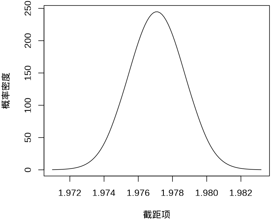
不难看出，截距项在 1.976 至 1.978 之间，50个参数的最大后验估计分别如下：

idx <- apply(rongelap_ginla$density, 1, function(x) x == max(x))
rongelap_ginla$beta[t(idx)]

#>  [1]  1.977019e+00 -5.124099e+02  5.461183e+03  1.515296e+03 -2.822166e+03
#>  [6] -1.598371e+04 -6.417855e+03  1.938122e+02 -4.270878e+03  3.769951e+03
#> [11] -1.002035e+04  1.914717e+03 -9.721572e+03 -3.794461e+04 -1.401549e+04
#> [16] -5.376582e+04 -1.585899e+04 -2.338235e+04  6.239053e+04 -3.574500e+02
#> [21] -4.587927e+04  1.723604e+04 -4.514781e+03  9.184026e-02  3.496526e-01
#> [26] -1.477406e+02  4.585057e+03  9.153647e+03  1.929387e+04 -1.116512e+04
#> [31] -1.166149e+04  8.079451e+02  3.627369e+03 -9.835680e+03  1.357777e+04
#> [36]  1.487742e+04  3.880562e+04 -1.708858e+03  2.775844e+04  2.527415e+04
#> [41] -3.932957e+04  3.548123e+04 -1.116341e+04  1.630910e+04 -9.789381e+02
#> [46] -2.011250e+04  2.699657e+04 -4.744393e+04  2.753347e+04  2.834356e+04

37.2.4 INLA

接下来，介绍完整版的近似贝叶斯推断方法 INLA — 集成嵌套拉普拉斯近似 (Integrated Nested Laplace Approximations，简称 INLA) (Rue, Martino, 和 Chopin 2009)。根据研究区域的边界构造非凸的内外边界，处理边界效应。

library(INLA)
library(splancs)
# 构造非凸的边界
boundary <- list(
  inla.nonconvex.hull(
    points = as.matrix(rongelap_coastline[,c("cX", "cY")]), 
    convex = 100, concave = 150, resolution = 100),
  inla.nonconvex.hull(
    points = as.matrix(rongelap_coastline[,c("cX", "cY")]), 
    convex = 200, concave = 200, resolution = 200)
)

根据研究区域的情况构造网格，边界内部三角网格最大边长为 300，边界外部最大边长为 600，边界外凸出距离为 100 米。

# 构造非凸的网格
mesh <- inla.mesh.2d(
  loc = as.matrix(rongelap[, c("cX", "cY")]), offset = 100,
  max.edge = c(300, 600), boundary = boundary
)

构建 SPDE，指定自协方差函数为指数型，则 \(\nu = 1/2\) ，因是二维平面，则 \(d = 2\) ，根据 \(\alpha = \nu + d/2\) ，从而 alpha = 3/2 。

spde <- inla.spde2.matern(mesh = mesh, alpha = 3/2, constr = TRUE)

生成 SPDE 模型的指标集，也是随机效应部分。

indexs <- inla.spde.make.index(name = "s", n.spde = spde$n.spde)
lengths(indexs)

#>       s s.group  s.repl 
#>     691     691     691

投影矩阵，三角网格和采样点坐标之间的投影。观测数据 rongelap 和未采样待预测的位置数据 rongelap_grid_df

# 观测位置投影到三角网格上
A <- inla.spde.make.A(mesh = mesh, loc = as.matrix(rongelap[, c("cX", "cY")]) )
# 预测位置投影到三角网格上
coop <- as.matrix(rongelap_grid_df[, c("cX", "cY")])
Ap <- inla.spde.make.A(mesh = mesh, loc = coop)
# 1612 个预测位置
dim(Ap)

#> [1] 1612  691

准备观测数据和预测位置，构造一个 INLA 可以使用的数据栈 Data Stack。

# 在采样点的位置上估计 estimation stk.e
stk.e <- inla.stack(
  tag = "est",
  data = list(y = rongelap$counts, E = rongelap$time),
  A = list(rep(1, 157), A),
  effects = list(data.frame(b0 = 1), s = indexs)
)

# 在新生成的位置上预测 prediction stk.p
stk.p <- inla.stack(
  tag = "pred",
  data = list(y = NA, E = NA),
  A = list(rep(1, 1612), Ap),
  effects = list(data.frame(b0 = 1), s = indexs)
)

# 合并数据 stk.full has stk.e and stk.p
stk.full <- inla.stack(stk.e, stk.p)

指定响应变量与漂移项、联系函数、模型公式。

# 精简输出
inla.setOption(short.summary = TRUE)
# 模型拟合
res <- inla(formula = y ~ 0 + b0 + f(s, model = spde),
  data = inla.stack.data(stk.full),
  E = E, # E 已知漂移项
  control.family = list(link = "log"),
  control.predictor = list(
    compute = TRUE, 
    link = 1, # 与 control.family 联系函数相同
    A = inla.stack.A(stk.full)
  ),
  control.compute = list(
    cpo = TRUE, 
    waic = TRUE, # WAIC 统计量 通用信息准则
    dic = TRUE   # DIC 统计量 偏差信息准则
  ),
  family = "poisson"
)
# 模型输出
summary(res)

#> Fixed effects:
#>     mean    sd 0.025quant 0.5quant 0.975quant  mode kld
#> b0 1.828 0.061      1.706    1.828      1.948 1.828   0
#> 
#> Model hyperparameters:
#>               mean    sd 0.025quant 0.5quant 0.975quant  mode
#> Theta1 for s  2.00 0.062       1.88     2.00       2.12  2.00
#> Theta2 for s -4.85 0.130      -5.11    -4.85      -4.59 -4.85
#> 
#> Deviance Information Criterion (DIC) ...............: 1834.57
#> Deviance Information Criterion (DIC, saturated) ....: 314.90
#> Effective number of parameters .....................: 156.46
#> 
#> Watanabe-Akaike information criterion (WAIC) ...: 1789.32
#> Effective number of parameters .................: 80.06
#> 
#>  is computed

• kld 表示 Kullback-Leibler divergence (KLD) 它的值描述标准高斯分布与 Simplified Laplace Approximation 之间的差别，值越小越表示拉普拉斯的近似效果好。

• DIC 和 WAIC 指标都是评估模型预测表现的。另外，还有两个量计算出来了，但是没有显示，分别是 CPO 和 PIT 。CPO 表示 Conditional Predictive Ordinate (CPO)，PIT 表示 Probability Integral Transforms (PIT) 。

固定效应（截距）和超参数部分

# 截距
res$summary.fixed

#>        mean         sd 0.025quant 0.5quant 0.975quant     mode          kld
#> b0 1.828027 0.06147353   1.706422 1.828284   1.948169 1.828279 1.782546e-08

# 超参数
res$summary.hyperpar

#>                   mean         sd 0.025quant  0.5quant 0.975quant      mode
#> Theta1 for s  2.000684 0.06235058   1.876512  2.001169   2.122006  2.003209
#> Theta2 for s -4.851258 0.12973385  -5.105061 -4.851807  -4.594253 -4.854093

提取预测数据，并整理数据。

# 预测值对应的指标集合
index <- inla.stack.index(stk.full, tag = "pred")$data
# 提取预测结果，后验均值
# pred_mean <- res$summary.fitted.values[index, "mean"]
# 95% 预测下限
# pred_ll <- res$summary.fitted.values[index, "0.025quant"]
# 95% 预测上限
# pred_ul <- res$summary.fitted.values[index, "0.975quant"]
# 整理数据
rongelap_grid_df$ypred <- res$summary.fitted.values[index, "mean"]
# 预测值数据
rongelap_grid_sf <- st_as_sf(rongelap_grid_df, coords = c("cX", "cY"), dim = "XY")
rongelap_grid_stars <- st_rasterize(rongelap_grid_sf, nx = 150, ny = 75)
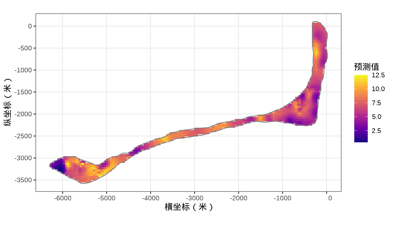
rongelap_stars <- st_crop(x = rongelap_grid_stars, y = rongelap_coastline_sfp)

最后，类似之前 mgcv 建模的最后一步，将 INLA 的预测结果绘制出来。

ggplot() +
  geom_stars(data = rongelap_stars, aes(fill = ypred), na.action = na.omit) +
  geom_sf(data = rongelap_coastline_sfp, fill = NA, color = "gray50", linewidth = 0.5) +
  scale_fill_viridis_c(option = "C") +
  theme_bw() +
  labs(x = "横坐标（米）", y = "纵坐标（米）", fill = "预测值")

图 37.11: 核辐射强度的预测分布

37.3 案例：城市土壤重金属污染

介绍多元地统计（Multivariate geostatistics）建模分析与 INLA 实现。分析某城市地表土壤重金属污染情况，找到污染最严重的地方，即寻找重金属污染的源头。

city_data <- readRDS(file = "data/cumcm2011A.rds")
library(sf)
city_data <- st_as_sf(city_data, coords = c("x(m)", "y(m)"), dim = "XY")
city_data

#> Simple feature collection with 319 features and 12 fields
#> Geometry type: POINT
#> Dimension:     XY
#> Bounding box:  xmin: 0 ymin: 0 xmax: 28654 ymax: 18449
#> CRS:           NA
#> First 10 features:
#>    编号 功能区 海拔(m) 功能区名称 As (μg/g) Cd (ng/g) Cr (μg/g) Cu (μg/g)
#> 1     1      4       5     交通区      7.84     153.8     44.31     20.56
#> 2     2      4      11     交通区      5.93     146.2     45.05     22.51
#> 3     3      4      28     交通区      4.90     439.2     29.07     64.56
#> 4     4      2       4     工业区      6.56     223.9     40.08     25.17
#> 5     5      4      12     交通区      6.35     525.2     59.35    117.53
#> 6     6      2       6     工业区     14.08    1092.9     67.96    308.61
#> 7     7      4      15     交通区      8.94     269.8     95.83     44.81
#> 8     8      2       7     工业区      9.62    1066.2    285.58   2528.48
#> 9     9      4      22     交通区      7.41    1123.9     88.17    151.64
#> 10   10      4       7     交通区      8.72     267.1     65.56     29.65
#>    Hg (ng/g) Ni (μg/g) Pb (μg/g) Zn (μg/g)          geometry
#> 1        266      18.2     35.38     72.35    POINT (74 781)
#> 2         86      17.2     36.18     94.59  POINT (1373 731)
#> 3        109      10.6     74.32    218.37 POINT (1321 1791)
#> 4        950      15.4     32.28    117.35    POINT (0 1787)
#> 5        800      20.2    169.96    726.02 POINT (1049 2127)
#> 6       1040      28.2    434.80    966.73 POINT (1647 2728)
#> 7        121      17.8     62.91    166.73 POINT (2883 3617)
#> 8      13500      41.7    381.64   1417.86 POINT (2383 3692)
#> 9      16000      25.8    172.36    926.84 POINT (2708 2295)
#> 10        63      21.7     36.94    100.41 POINT (2933 1767)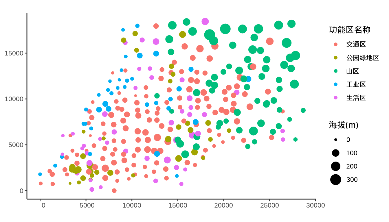

ggplot(data = city_data) +
  geom_sf(aes(color = `功能区名称`, size = `海拔(m)`)) +
  theme_classic()

图 37.12: 某城市的地形

library(ggplot2)
ggplot(data = city_data) +
  geom_sf(aes(color = `功能区名称`, size = `As (μg/g)`)) +
  theme_classic()
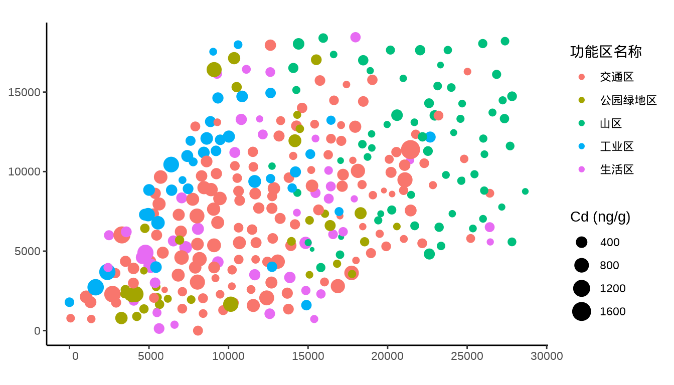
ggplot(data = city_data) +
  geom_sf(aes(color = `功能区名称`, size = `Cd (ng/g)`)) +
  theme_classic()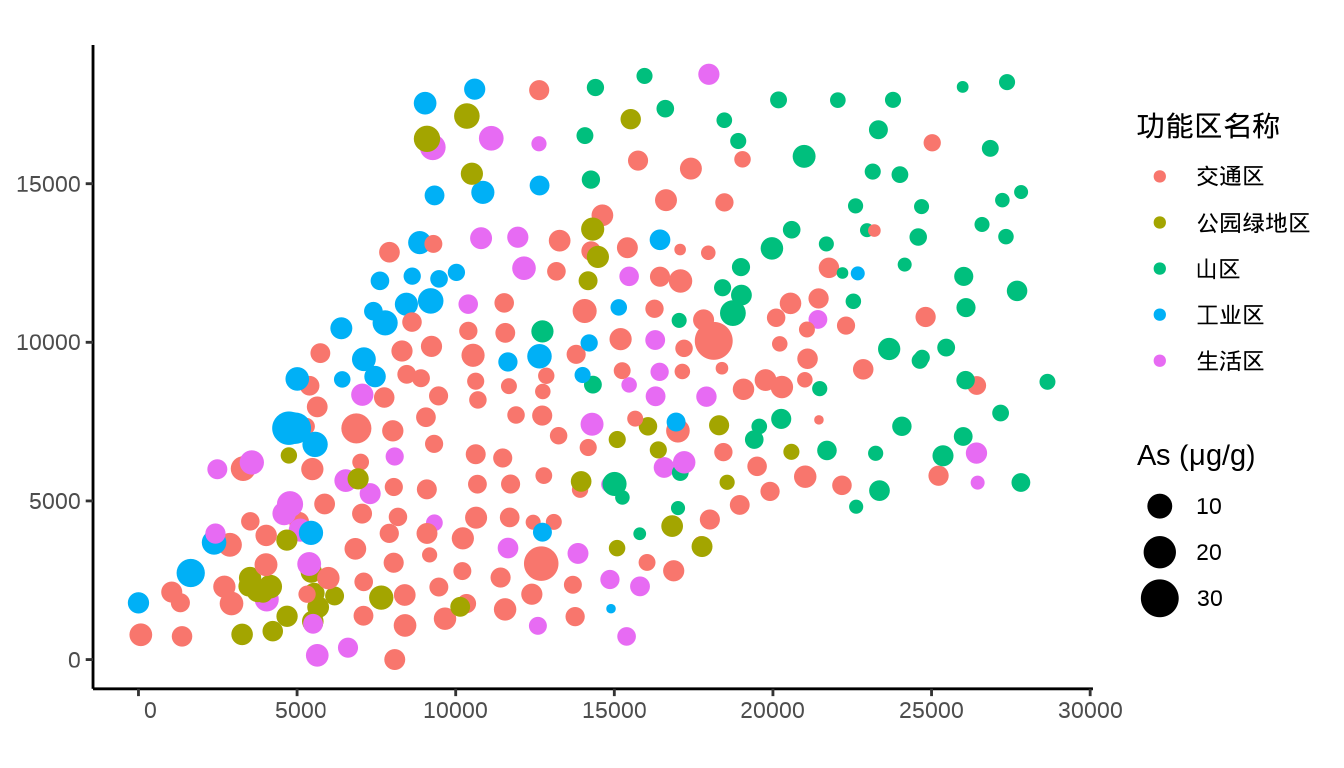

(a) 重金属砷 As

(b) 重金属镉 Cd

图 37.13: 重金属砷 As 和镉 Cd 的浓度分布

为了便于建模，对数据做标准化处理。

# 根据背景值将各个重金属浓度列进行转化
city_data <- within(city_data, {
  `As (μg/g)` <- (`As (μg/g)` - 3.6) / 0.9
  `Cd (ng/g)` <- (`Cd (ng/g)` - 130) / 30
  `Cr (μg/g)` <- (`Cr (μg/g)` - 31) / 9
  `Cu (μg/g)` <- (`Cu (μg/g)` - 13.2) / 3.6
  `Hg (ng/g)` <- (`Hg (ng/g)` - 35) / 8
  `Ni (μg/g)` <- (`Ni (μg/g)` - 12.3) / 3.8
  `Pb (μg/g)` <- (`Pb (μg/g)` - 31) / 6
  `Zn (μg/g)` <- (`Zn (μg/g)` - 69) / 14
})

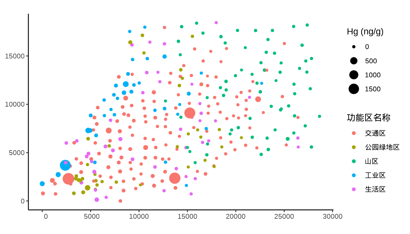
当我们逐一检查各个重金属的浓度分布时，发现重金属汞 Hg 在四个地方的浓度极高，暗示着如果数据采集没有问题，那么这几个地方很可能是污染源。

ggplot(data = city_data) +
  geom_sf(aes(color = `功能区名称`, size = `Hg (ng/g)`)) +
  theme_classic()

图 37.14: 重金属汞 Hg 的浓度分布

37.3.1 mgcv

mgcv 包用于基于惩罚似然的多元模型平滑参数估计和选择 (Simon N. Wood, Pya, 和 Säfken 2016)。

# ?mvn

37.3.2 INLA

INLA 包用于多元空间模型的贝叶斯推断 (Palmí-Perales 等 2022) 。

Palmí-Perales, Francisco, Virgilio Gómez-Rubio, Roger S. Bivand, Michela Cameletti, 和 Håvard Rue. 2022. 《Bayesian Inference for Multivariate Spatial Models with R-INLA》. The R Journal. https://doi.org/10.48550/arXiv.2212.10976.

Rasmussen, Carl Edward, 和 Christopher K. I. Williams. 2006. Gaussian Processes for Machine Learning. Cambridge, Massachusetts: MIT Press. https://gaussianprocess.org/gpml/.

Rue, Håvard, Sara Martino, 和 Nicholas Chopin. 2009. 《Approximate Bayesian Inference for Latent Gaussian Models Using Integrated Nested Laplace Approximations (with discussion)》. Journal of the Royal Statistical Society, Series B 71 (2): 319–92.

Sainsbury-Dale, Matthew, Andrew Zammit-Mangion, 和 Noel Cressie. 2022. 《Modelling Big, Heterogeneous, Non-Gaussian Spatial and Spatio-Temporal Data using FRK》. Journal of Statistical Software. https://doi.org/10.48550/arXiv.2110.02507.

Wood, S. N. 2004. 《Stable and efficient multiple smoothing parameter estimation for generalized additive models》. Journal of the American Statistical Association 99 (467): 673–86.

Wood, Simon N. 2019. 《Simplified integrated nested Laplace approximation》. Biometrika 107 (1): 223–30. https://doi.org/10.1093/biomet/asz044.

Wood, Simon N., Natalya Pya, 和 Benjamin Säfken. 2016. 《Smoothing Parameter and Model Selection for General Smooth Models》. Journal of the American Statistical Association 111 (516): 1548–63. https://doi.org/10.1080/01621459.2016.1180986.